What does it mean to not have a “mean”? — Working with fat-tailed distributions

Many traders instinctively look to the mean for value and variance for risk, but there are good reasons why these statistics are not always the most appropriate.
The log returns of an exchange traded asset generally show a smooth, unimodal distribution, and it is natural to look to the mean for an estimate of value, and the variance to estimate risk. These values are easily calculated from sample data, but it is important to consider how informative they are when it comes to understanding the underlying distribution.
Additionally, market returns are known to be fat-tailed, and failing to properly account for this can lead to drastically underestimating the likelihood of extreme events — as LTCM and others have found out to their cost.
The family of ⍺-stable distributions range from the Gaussian, through increasingly fat-tailed distributions, and naturally incorporate skew. They model financial data well, but there are some remarkable implications for the choice of summary statistics, since, for all but the Gaussian, the variance is undefined, and when the tails are sufficiently fat, even the mean is undefined!
Stable distributions
Stable distributions have been used to analyse financial data at least since Benoit Mandelbrot, of fractal fame, wrote on this as early as 1963.
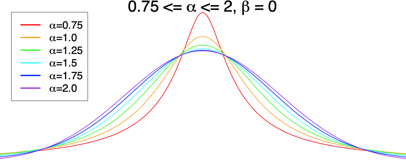
The family of ⍺-stable distributions have their shape determined by a parameter ⍺, starting at 2 for a Gaussian, and producing increasingly fat tails as it decreases to 0.
The tails are asymptotically proportional to a power law.

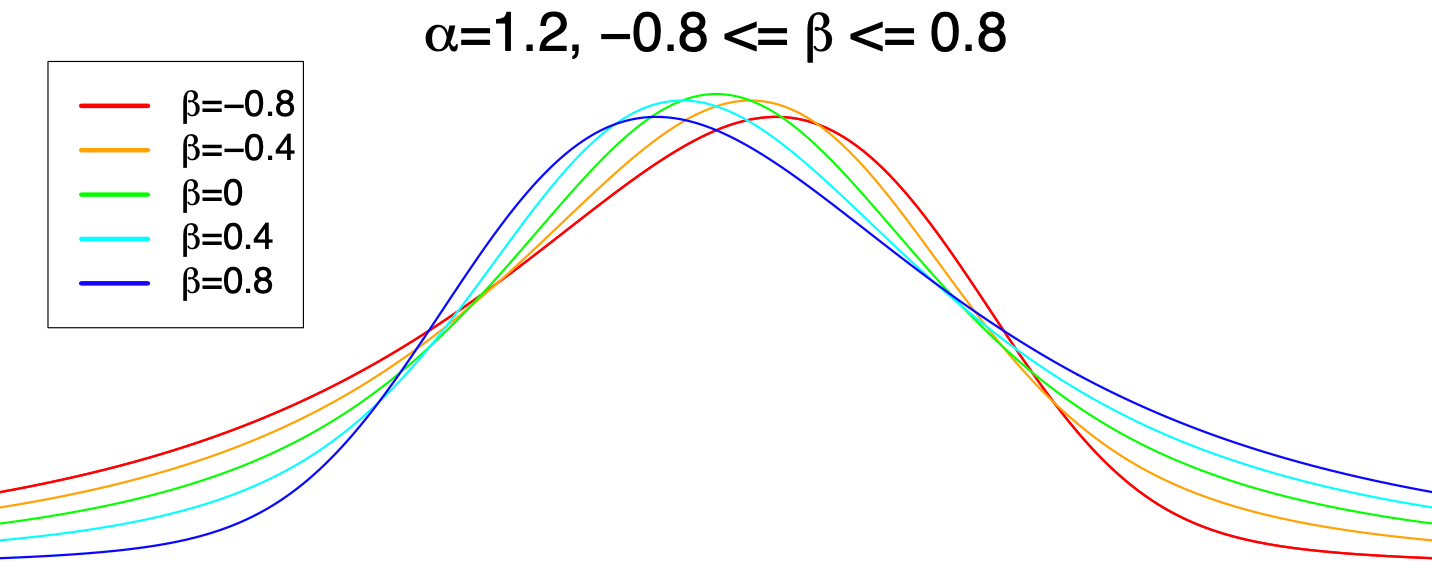
A second parameter, β, that ranges between +/-1, determines the skew of the distribution. When ⍺ = 2 this has no effect, but as ⍺ decreases, the introduced skew becomes more pronounced.

Analysing samples from a stable distribution
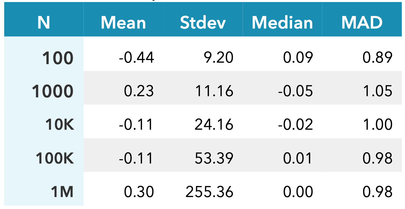
Let’s generate some random samples from a symmetric stable distribution with ⍺ = 1.2, and calculate the sample mean and deviation. As the table below shows, even up to 1 million samples, the mean remains unclear, and the deviation does not converge.

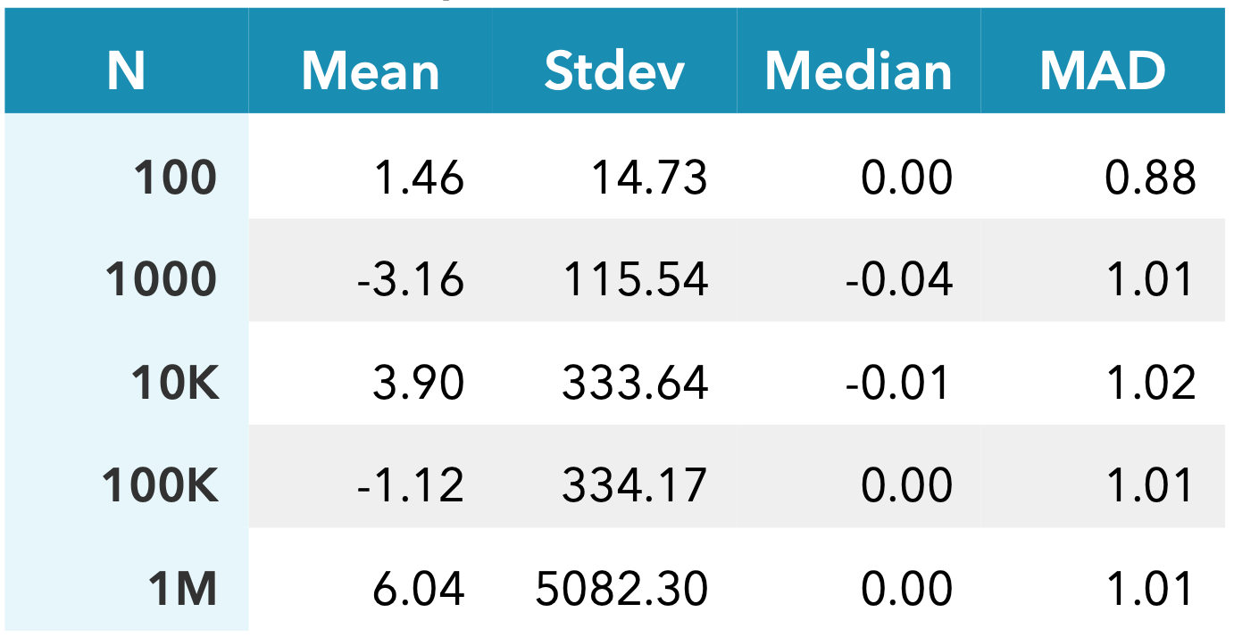
If we fatten the tails further by reducing ⍺ to 0.95, even the mean fails to converge.

Clearly, these measures are not providing meaningful information about the underlying distribution.
How can this be overcome?
Replacing the mean and standard deviation by the corresponding robust measures, the median and median absolute deviation (MAD), results in the values shown opposite for the ⍺ = 1.2 samples.

Both these measures converge nicely, and are effective alternatives.
As the second table shows, they remain effective with the fatter tails of ⍺ = 0.95.

In the presence of skew, the median and MAD are able to capture and quantify the central shift and width of the distribution, as seen below when ⍺ = 1.4, β = 0.6

What about real market data?
The following chart shows 1 day of BHP trading on the ASX. The corresponding histogram of 2 minute returns includes a stable distribution fit with ⍺ = 1.5, β = 0.24.

Next are the same charts for 1 day of trading of BTCUSD. The stable distribution fit has ⍺ = 1.64, β = 0.04.

It is clear that the stable distribution is quite successful in recognising the fat tails, much more so than a Gaussian, and hence modelling with these distributions is better suited for capturing the associated extra risk.